WHAT IT IS

An MRI machine (magnetic resonance imaging scanner, originally called an NMR imager for nuclear magnetic resonance) makes cross-sectional and 3D images of the inside of the body using a very strong static magnetic field, changing magnetic field gradients and pulses of radio waves. It uses no X-rays and no ionizing radiation. The signal comes mostly from hydrogen nuclei (single protons) in water and fat, which makes the method superb at showing soft tissue: brain, spinal cord, muscle, ligament, cartilage, liver, prostate, heart and blood vessels.

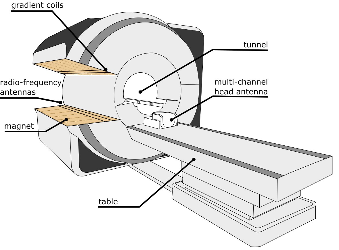
The machine is a large tube (the bore) built around a powerful magnet, usually 60 to 70 cm across in a conventional scanner, with a motorized patient table that slides the patient into the middle. Hidden inside the bore wall are the gradient coils and the radio-frequency (RF) body coil. Local receive coils, shaped for the head, knee, spine, breast and so on, are placed on or around the part being scanned. Around the whole thing is an RF-shielded room, and in the next room is the operator console and the electronics cabinets.

MRI is a physics-rich, flexible method: the same machine can be made to show anatomy, water diffusion, blood flow, brain activation, iron deposits, fat fraction or chemical composition simply by changing the pulse sequence (the timing program). It is slower and louder than CT, and the magnet is always on, which creates its own safety rules, but for most soft-tissue questions it gives the best contrast of any imaging method.

HISTORY

Nuclear magnetic resonance. In 1938 Isidor Rabi measured nuclear magnetic resonance in molecular beams (Nobel Prize in Physics 1944). In 1946 two groups, Felix Bloch at Stanford and Edward Purcell at Harvard, independently detected NMR in bulk matter (liquids and solids), and shared the 1952 Nobel Prize in Physics. For the next few decades NMR was a laboratory chemistry tool used to identify molecules; it produced spectra, not pictures. Electron paramagnetic (spin) resonance, a related effect for unpaired electrons, was discovered by Yevgeny Zavoisky in 1944.

Raymond Damadian. In 1971 the American physician and scientist Raymond Damadian published a paper in Science reporting that the NMR relaxation times (T1 and T2) of some tumor tissue in rats were longer than those of normal tissue. This suggested NMR could tell diseased tissue from healthy tissue. He filed a patent in 1972 for an NMR-based cancer detection apparatus, and in 1977 his team (Damadian, Larry Minkoff and Michael Goldsmith) scanned a human chest with a superconducting-magnet machine they called Indomitable. That first scan reportedly took several hours (commonly quoted as about four to five hours) and moved the patient step by step so a single small spot at a time was measured. He founded FONAR in 1978, which sold some of the first commercial MRI scanners.

Paul Lauterbur. In 1973 the American chemist Paul Lauterbur, at Stony Brook, published in Nature the idea of making an image by superimposing a magnetic field gradient on the main field, so that the resonance frequency depends on position. He called the technique zeugmatography (from the Greek for "that which joins together"), and showed images of two small tubes of water. This is the key idea that turned NMR into imaging.

Peter Mansfield. At the University of Nottingham, Peter Mansfield developed the mathematical and practical use of gradients to encode and select slices, and showed how signals could be analyzed quickly. In 1977 he proposed echo-planar imaging (EPI), which can collect a whole image in a fraction of a second after one excitation. EPI was not practical on clinical machines until gradient hardware improved in the late 1980s and 1990s, but today it is the basis of functional and diffusion MRI. His group also produced early human images, such as of a finger in 1977 and later of the abdomen.

The practical imaging method. A group at Aberdeen (Hutchison, Mallard, Edelstein and colleagues) built early whole-body scanners around 1980 and in 1980 published the spin-warp technique, a Fourier imaging method using phase-encoding gradients. Spin-warp, with later variations, is the basis of most clinical MRI sequences today.

The 2003 Nobel Prize. The 2003 Nobel Prize in Physiology or Medicine was awarded to Paul Lauterbur and Peter Mansfield "for their discoveries concerning magnetic resonance imaging". Raymond Damadian was not included, which was publicly disputed (he took out full-page newspaper advertisements protesting it). Credit for the invention of MRI remains a point of argument; the commonly accepted view is that Damadian showed the medical principle, Lauterbur invented gradient-based imaging, and Mansfield made it fast and mathematically practical.

Commercialization. Commercial whole-body MRI scanners appeared in the early 1980s from several firms, including FONAR, Picker, Technicare, General Electric, Siemens, Philips and others (exact first-sale dates differ between sources). The US FDA approved MRI for clinical use in 1985. GE Signa 1.5 T and Siemens Magnetom 1.5 T systems of the early to mid 1980s established the 1.5 tesla superconducting scanner as the standard hospital machine for decades. The first gadolinium-based contrast agent (gadopentetate dimeglumine, Magnevist) was approved around 1988. Name changes marked the era: the word "nuclear" was dropped from the public name (NMR imaging became MRI) partly because of public worry about the word.

Later milestones. Diffusion MRI developed in the mid 1980s (Denis Le Bihan and others). Functional MRI using the BOLD effect appeared in 1990 to 1992 (Seiji Ogawa; Kenneth Kwong and colleagues). Diffusion tensor imaging was described in 1994 (Peter Basser and colleagues). 3 T became common in hospitals in the 2000s, and 7 T whole-body systems received clinical clearance (US FDA, Siemens Magnetom Terra) in 2017. Since the 2010s there have been sealed low-helium magnets, wide bores of 70 to 80 cm, deep-learning image reconstruction and portable low-field scanners.

PHYSICS: HOW AN IMAGE IS BUILT

Spin and magnetization. A hydrogen nucleus is a single proton with a property called spin, which makes it behave like a tiny bar magnet. In normal life the magnets point in random directions. In the strong static field of the scanner, called B0, they line up slightly with it (a few more parallel than anti-parallel). The surplus is tiny, roughly 5 to 10 in a million at clinical field strengths (approximate), but there are so many protons in a body (on the order of 10 to the 27th or 28th hydrogen atoms in a human, roughly) that the sum is measurable. This net magnetization points along B0 (the z axis).

Larmor frequency. Each proton precesses (wobbles like a spinning top) around B0 at the Larmor frequency, which is proportional to field strength: f = gamma x B0. For hydrogen, gamma divided by 2 pi is about 42.58 MHz per tesla. So at 1.5 T the frequency is about 63.9 MHz, at 3 T about 127.7 MHz, and at 7 T about 298 MHz. These are radio frequencies, in the range of VHF television and FM-band radio.

RF excitation. A short pulse of RF energy at the Larmor frequency, transmitted by the body coil, tips the net magnetization away from the z axis by a chosen flip angle (for example 90 degrees or smaller). Only protons whose frequency matches the pulse respond: this is the resonance. After the pulse the tilted magnetization precesses in the transverse plane, and a precessing magnet induces a voltage in a nearby coil, the way a generator does. That voltage, a decaying oscillation at the Larmor frequency, is the free induction decay (FID) and is the MR signal.

Relaxation: T1, T2 and T2*. After excitation the protons return to equilibrium in two ways at once. T1 (longitudinal or spin-lattice relaxation) is the time constant for the magnetization to regrow along z, as the protons give energy back to their surroundings. T2 (transverse or spin-spin relaxation) is the time constant for the signal in the transverse plane to decay as the protons lose phase coherence by interacting with each other. T2* is the faster decay that also includes dephasing from field inhomogeneity, so T2* is always shorter than T2. Different tissues have different values, and that difference is the basis of contrast. Typical approximate values at 1.5 T: fat T1 about 250 ms, white matter about 600 ms, gray matter about 900 ms, cerebrospinal fluid (CSF) several seconds; T2 of brain tissue about 70 to 100 ms and of CSF around 2000 ms. T1 values lengthen at higher field and T2 shortens slightly. These are textbook ranges, not exact.

Proton density. The raw signal strength also depends on how many mobile hydrogen nuclei are in the voxel. Lung and cortical bone have few and show almost no signal, which is why they are dark on MRI. Water-rich tissue and fat give lots.

Spin echo. In a spin-echo sequence a 90 degree excitation is followed, after time TE/2, by a 180 degree refocusing pulse, which reverses the dephasing caused by static field inhomogeneity. The signal re-forms into an echo at time TE (echo time), and what has decayed by then is the true T2 decay. Fast (turbo) spin echo collects many echoes after one excitation and is the workhorse for T2-weighted images.

Gradient echo. A gradient-echo sequence uses a partial flip angle (for example 10 to 40 degrees) and re-forms the echo with a reversal of a gradient instead of a 180 degree pulse. It is faster, but is sensitive to field inhomogeneity (T2* weighting), which is a disadvantage for metal and air-tissue boundaries and an advantage for detecting blood products and iron.

Slice selection, frequency encoding and phase encoding. Without extra information every proton in the body would ring at the same frequency, and there would be no image. The gradient coils add a linear field change across the bore, so the frequency becomes position dependent. Three steps are used:

• Slice selection: a gradient is switched on while the RF pulse is sent, so only a slice with the matching frequency band is excited. Slice thickness depends on the gradient strength and the pulse bandwidth.
• Frequency encoding: a gradient is on while the signal is read out, so position along one axis is encoded as frequency.
• Phase encoding: a short gradient applied before the readout leaves protons at different positions along the other axis at different phase angles. This is repeated with a different phase-encoding step for each line of the image (one line per TR in a basic sequence).

k-space and the Fourier transform. The raw data are stored in a matrix called k-space, which is not the image but its spatial-frequency representation. The center of k-space holds the low spatial frequencies, which set overall contrast and signal; the edges hold high spatial frequencies, which give sharp detail and edges. A two-dimensional (or three-dimensional) inverse Fourier transform turns k-space into the image. Almost every modern speed-up (parallel imaging such as SENSE and GRAPPA, compressed sensing, partial Fourier, simultaneous multi-slice, deep-learning reconstruction) works by under-sampling k-space cleverly and filling in the missing data.

TR, TE and weighting. TR (repetition time) is the time between successive excitations; TE (echo time) is the time from excitation to the echo. Choosing them selects the contrast:

• T1-weighted: short TR and short TE. Fat is bright, fluid is dark. Good anatomy, and post-contrast images (gadolinium shortens T1 and brightens enhancing tissue).
• T2-weighted: long TR and long TE. Fluid is bright, so edema, cysts, fluid-filled lesions and CSF stand out.
• Proton-density (PD) weighted: long TR and short TE. Common for knee cartilage and menisci.
• FLAIR (fluid-attenuated inversion recovery): a T2-weighted image with an inversion pulse timed to null the CSF signal, so lesions near the ventricles and cortex (for example multiple sclerosis plaques) are not hidden by the bright fluid.
• STIR (short-tau inversion recovery) and fat-saturated sequences suppress fat signal so that edema and fluid in fatty tissue show.
• DWI (diffusion-weighted imaging) and ADC (apparent diffusion coefficient map): sensitized to the random motion of water. Strong gradient pulses make signal drop where water moves freely; restricted diffusion (for example in acute stroke cells that have swollen) stays bright on DWI and dark on the ADC map. DWI can show an acute infarct within minutes to an hour or so of onset, much earlier than CT.
• SWI (susceptibility-weighted imaging): a high-resolution gradient-echo method that shows small bleeds (microhemorrhages), veins, calcium and iron.

MR angiography (MRA). Blood vessels can be imaged with and without contrast. Time-of-flight (TOF) uses the fact that fresh unsaturated blood flowing into a slice gives more signal than the stationary tissue that has been repeatedly excited. Phase-contrast MRA uses the phase shift of moving protons and can measure flow velocity. Contrast-enhanced MRA injects gadolinium and images fast while it is in the arteries.

Functional MRI (fMRI). The most common method relies on the BOLD (blood-oxygen-level-dependent) effect. Deoxygenated hemoglobin is paramagnetic and shortens T2*; when a brain region becomes active, blood flow rises more than oxygen use, so there is less deoxyhemoglobin and the T2*-weighted signal rises slightly (a few percent at most at clinical fields). Echo-planar imaging collects whole-brain volumes every one to a few seconds, and statistics are used to find which areas change with a task or at rest. It measures blood response, not neurons directly.

Diffusion tensor imaging (DTI) and tractography. Water in white matter diffuses more easily along nerve fibers than across them. By measuring diffusion in at least six directions, a tensor can be calculated for each voxel, and from it come fractional anisotropy maps and fiber-tract reconstructions (tractography) used in neurosurgical planning and research.

MR spectroscopy (MRS). The exact resonance frequency of a proton depends slightly on the molecule it is in (chemical shift, in parts per million). MRS records a spectrum from a chosen region and shows metabolites such as N-acetylaspartate (NAA, a neuron marker), choline (raised in many tumors), creatine and lactate. It is used in brain tumor and metabolic work, and in prostate, and in research.

Other contrast mechanisms. Perfusion imaging (arterial spin labeling, or dynamic contrast), elastography (shear waves through the liver), fat and iron quantification (Dixon methods, R2*), magnetization transfer, and hyperpolarized-xenon or carbon-13 research for the lungs and metabolism all use the same hardware with different programs.

HARDWARE: THE MAGNET

Superconducting magnet. Almost all hospital scanners at 1.5 T and above use a superconducting electromagnet. The coil windings are a niobium-titanium (NbTi) alloy in a copper matrix, wound on a former and kept at about 4 K (around minus 269 C, close to absolute zero), usually by being bathed in liquid helium inside a vacuum-insulated vessel called the cryostat. At this temperature the wire has essentially zero resistance. After the magnet is brought up to field (ramped), the ends are joined with a superconducting switch and the current circulates in persistent mode for years without a power supply, so the field stays stable to a few parts per million per hour or better. A typical 1.5 T whole-body magnet weighs several tonnes (roughly 4 to 7 tonnes for the magnet alone, approximate) and 3 T and higher magnets weigh more.

Cryogenics and the cold head. Heat leaking in would boil the helium. A cryocooler (a two-stage Gifford-McMahon type, whose cold part is called the cold head) mounted on the cryostat recondenses helium vapor back to liquid, working 24 hours a day, so a modern magnet loses almost no helium in normal operation. The cold head compressor is a separate unit, water or air cooled, and the pulsing "chug" sound near some magnets is the cold head. Older magnets without a recondenser needed topping up every few months and burned a lot of helium. A traditional magnet holds on the order of 1,500 to 2,000 liters of liquid helium (approximate; depends on model).

Sealed low-helium magnets. Newer designs hold far less helium in a sealed system with no need to be refilled during life. Philips introduced its BlueSeal 1.5 T magnet around 2018 with about 7 liters of helium (according to the company), and Siemens Healthineers introduced the Magnetom Free.Max 0.55 T (about 0.7 liters) and later "DryCool" magnets. GE HealthCare and others have also announced low-helium or sealed designs. Helium is a finite resource that has had supply shortages and price spikes, which has driven this trend.

Quench. A quench is when the superconductor suddenly goes normal (resistive) and the stored magnetic energy turns into heat, boiling off the helium in a minute or less. It can be triggered by a fault, a loss of cooling, or deliberately by the emergency stop button when someone is pinned by metal or in danger. The helium turns to gas and expands roughly 700-fold (approximate), so the cryostat has a quench pipe (vent) that leads the cold gas safely to the outside of the building, and rupture discs protect the vessel. A quench is not a danger of explosion to the patient, but it releases a lot of cold gas that can displace oxygen in a room if the pipe is blocked or leaks, which is why rooms have oxygen monitors and the vent has to be well designed. After a quench the magnet has to be re-filled with helium and ramped to field again, which takes days and often costs tens of thousands of dollars (approximate), and may damage the magnet.

Actively shielded magnets. Modern superconducting magnets have a second set of oppositely wound coils outside the main coils to cancel the stray (fringe) field, which shrinks the area around the scanner where the field is strong. Older unshielded magnets needed tonnes of iron in the walls.

Permanent and resistive magnets. Low field open scanners use either a permanent magnet (large blocks of rare-earth alloy or ferrite on an iron yoke, always on, with no cryogens and no power use for the field) or a resistive electromagnet (copper coils that draw tens of kilowatts and need to be cooled). Typical fields are about 0.2 to 0.7 T (some permanent-magnet designs reach about 1.2 T). Open C-shaped or "double doughnut" designs reduce claustrophobia, allow larger or standing patients, and were used for interventional work. Image quality and speed are lower because signal rises with field strength. Very low field portable systems (for example the 64 mT Hyperfine Swoop, cleared by the US FDA in 2020) use permanent magnets and can be wheeled to the bedside.

Field strengths. Field strength is measured in tesla (T); the Earth's field is about 0.00005 T (50 microtesla). Typical classes:

• 0.2 to 0.7 T: open and low-field scanners.
• 1.5 T: the long-standing standard, robust, with lower artifacts and heating.
• 3 T: common in large hospitals and brain and research work. About double the signal of 1.5 T, but more susceptibility artifacts, more RF heating (SAR) and more noise.
• 7 T: ultra-high field. Whole-body 7 T research scanners have existed since the early 2000s, and one model was cleared for clinical use by the US FDA in 2017. Excellent brain detail, but difficult RF uniformity.
• 9.4 T and above: research only. 9.4 T human systems exist at several institutes; the 10.5 T system at the University of Minnesota and the 11.7 T "Iseult" system of CEA in France (first human images reported in 2024) are among the strongest human scanners built. Higher fields (14 T) are being planned. Small-animal research scanners go to 21 T and beyond (approximate).

Bore size. Conventional bores are 60 cm; "wide-bore" systems are 70 cm, and some are 75 to 80 cm (for example Siemens Free.Max at 80 cm, United Imaging models at 75 cm). The shorter the magnet and the bigger the bore, the harder it is to keep the field uniform. The ISO center (the point at the middle where the field is most uniform) is usually quoted as a sphere of about 40 to 50 cm.

Shim coils. The main field must be uniform to a few parts per million over the imaging volume, which the winding alone cannot achieve. Passive shimming uses small pieces of steel placed at set positions in trays inside the magnet bore; active shim coils (resistive, in the bore wall) correct the rest, and a patient-specific shim is run before each scan because the body itself distorts the field.

HARDWARE: GRADIENTS, RF AND ELECTRONICS

Gradient coils. Three sets of coils (X, Y and Z) inside the bore wall make the linear field variations used for slice selection and for frequency and phase encoding. They are driven by powerful gradient amplifiers that can deliver hundreds of amperes at over a thousand volts. Two key specifications: gradient strength, in millitesla per meter (clinical systems about 20 to 45 mT/m, some high-performance systems 80 mT/m, and a research system with 300 mT/m, the Connectom at Massachusetts General Hospital), and slew rate, how fast the gradient can ramp, in tesla per meter per second (typically 100 to 200 T/m/s, approximate). Stronger and faster gradients enable thinner slices, faster EPI and better diffusion imaging, but are limited by nerve stimulation.

Acoustic noise. The gradient coils sit in the static field, and a current in a wire in a field gives a force (the Lorentz force). Fast switching makes the coils flex and bang, which is the loud knocking and buzzing of a scan. Sound levels can exceed 100 dB, with some sequences reaching above 110 dB (approximate), so patients get earplugs or headphones. Quieter sequences and vacuum-isolated coil designs reduce it.

RF body coil. A large birdcage coil built into the bore wall transmits the RF excitation pulses to the whole body at the Larmor frequency and may also receive. At 3 T and above, more than one transmit channel (parallel transmit) is often used to even out the RF field.

Surface and phased-array coils. Receive-only coils close to the body pick up much more signal than the distant body coil. Common types include the head coil (often 8 to 64 channels), neurovascular coil, spine, knee, shoulder, wrist, breast, cardiac and flexible body "blanket" coils. Phased arrays of many small coil elements, each with its own receiver channel, allow parallel imaging (SENSE, GRAPPA) to speed up scans. Modern scanners have 32 to 128 or more receive channels. In the labeled diagram above, the multi-channel head antenna is one such coil.

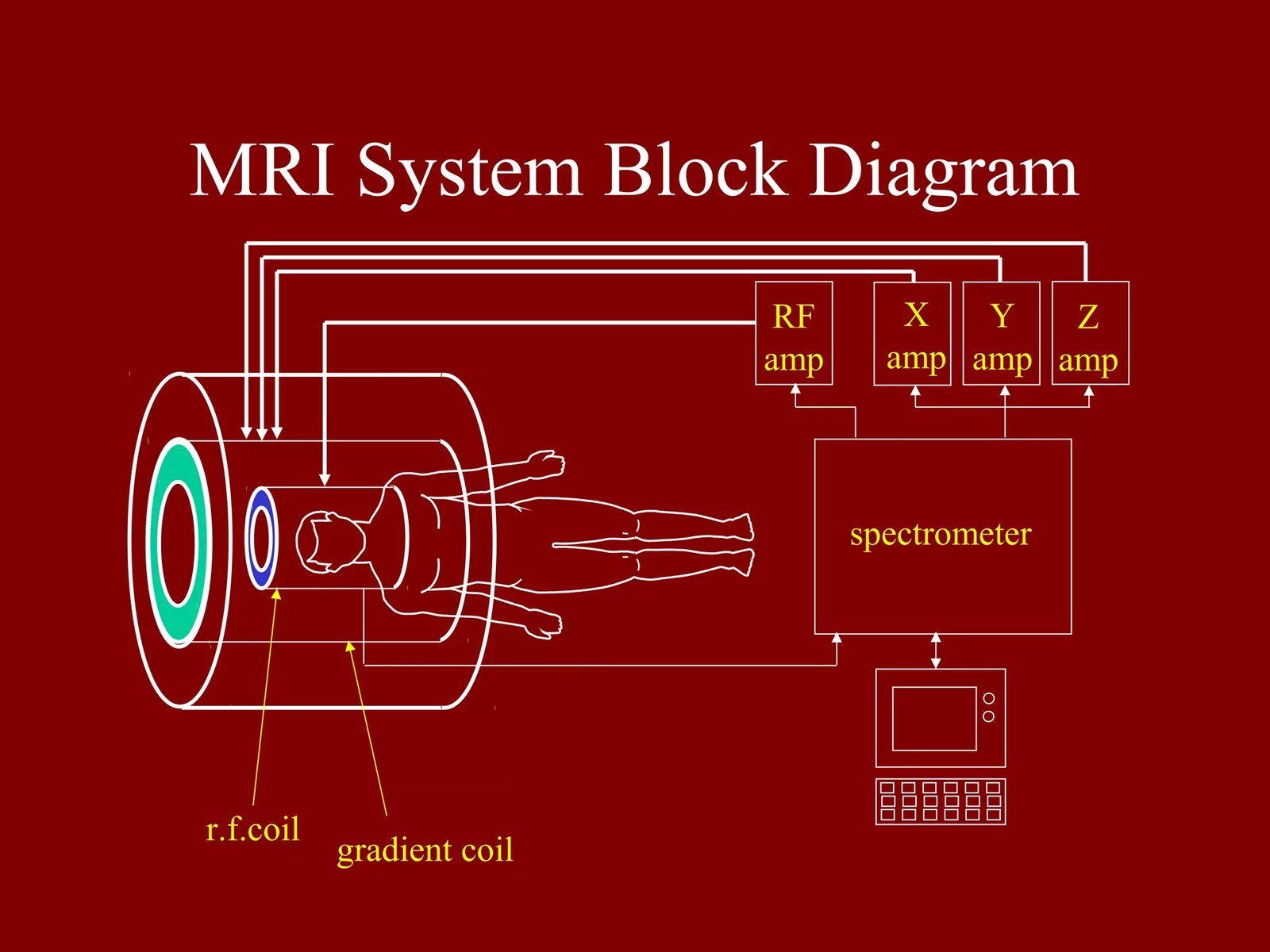
RF chain and spectrometer. The console computer sends the timing program to the spectrometer, which makes the precisely timed RF waveform (at the Larmor frequency, with a shaped envelope) and the gradient waveforms. The RF is amplified by a power amplifier (typically 15 to 35 kW peak for 1.5 T and 3 T body transmit, approximate) and goes to the transmit coil. The tiny received signal (microvolt level) passes through low-noise preamplifiers close to the coil, down-conversion to a lower frequency and digitization by analog-to-digital converters, then goes to the reconstruction computer. Modern systems digitize in or very near the coil, replacing long analog cables with fiber optic links.

Table and monitoring. The patient table is nonmagnetic and often detachable, with a motor drive and a laser or light positioning system. Patients have a squeeze ball alarm, an intercom, and sometimes ECG, respiration and pulse sensors for gating. Heart MRI needs ECG triggering and MR-conditional monitors.

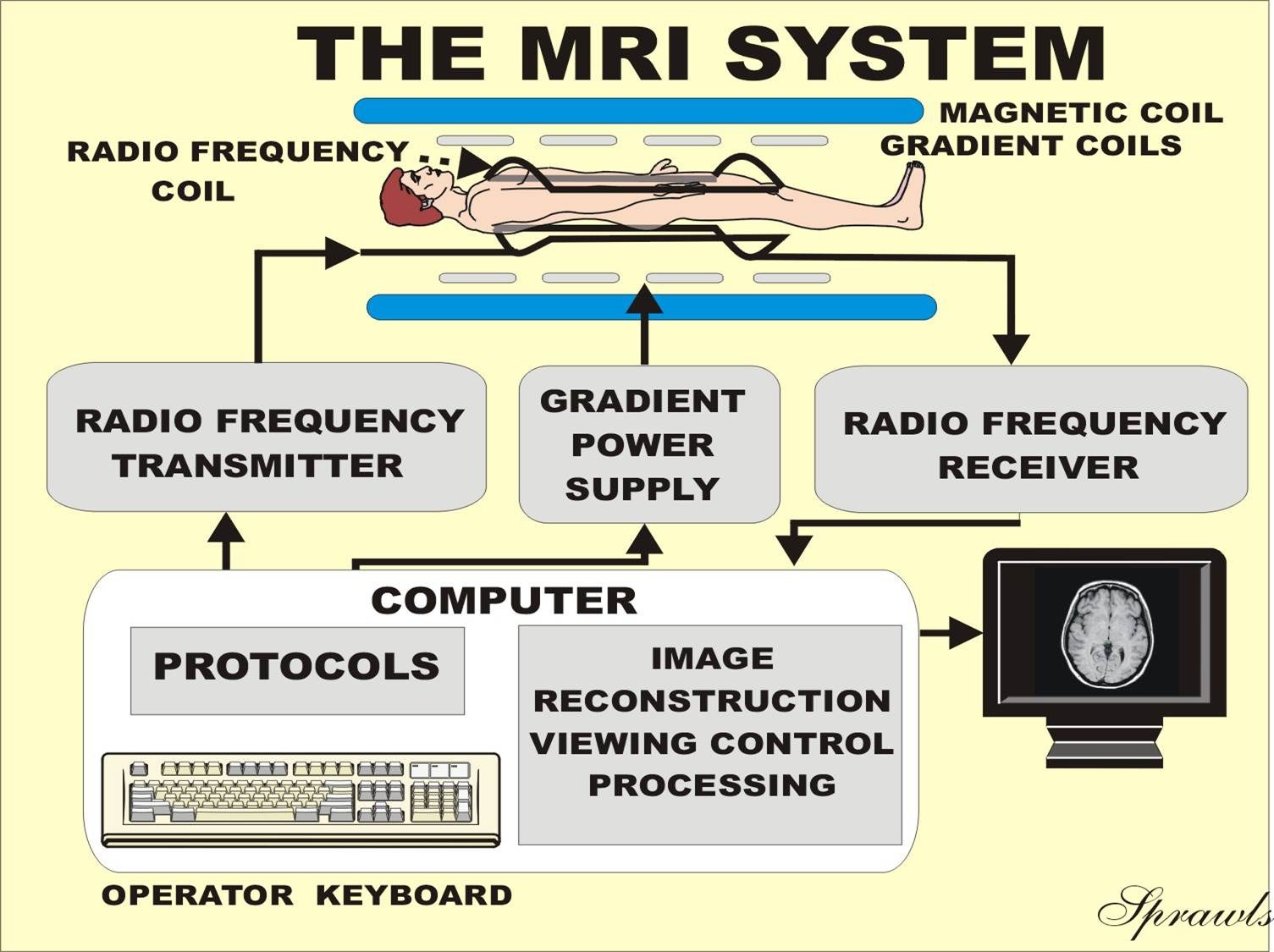
Computer and software. A host computer runs the protocols (stored sequences with parameters), a reconstruction computer with powerful graphics processors does the Fourier transform and parallel-imaging math, and images go to the hospital archive (PACS) as DICOM files. Block diagrams such as the ones shown at the top of this page summarize the system: computer, RF transmitter and receiver, gradient power supply, and the magnet, gradient and RF coils around the patient.

BLOCK DIAGRAM IN BRIEF

• Operator console and protocols: select sequence and parameters.
• Spectrometer / sequencer: generates the RF and gradient timing.
• RF power amplifier and transmit coil: excites the protons.
• X, Y and Z gradient amplifiers and gradient coils: spatial encoding.
• Magnet (B0) and shim coils: the static field.
• Receive coils, preamplifiers and digitizer: pick up the signal.
• Reconstruction computer: Fourier transform to image, then display and archive.

SAFETY

MRI contains no ionizing radiation, but it has serious hazards of its own, and most come from the fact that the magnet is always on, even when no scan is happening.

• Projectile (missile) effect: ferromagnetic objects (oxygen cylinders, wheelchairs, floor buffers, scissors, tools, IV poles) are pulled toward the magnet with great force and speed and can seriously injure or kill a person in the bore. There have been fatal accidents, including a 2001 case in the United States where a child was killed by an oxygen cylinder. Rooms use ferromagnetic detectors and strict screening.
• Implants and devices: pacemakers, defibrillators, cochlear implants, aneurysm clips, neurostimulators, insulin pumps and metal fragments in the eye can be dangerous. Items are labeled MR Safe, MR Conditional (safe only under stated conditions such as field strength, gradient and SAR limits) or MR Unsafe. Many modern pacemakers are MR Conditional, but they require a specific protocol and monitoring. Patients are screened by questionnaire and sometimes radiographs.
• RF heating and SAR: the RF energy warms tissue. The specific absorption rate (SAR) in watts per kilogram is monitored by the scanner, and limits are set by standards (for example the IEC limits of about 2 W/kg whole-body in normal operating mode and 4 W/kg in first-level mode, approximate). Conductive loops, leads and some tattoos or metal can cause local burns, so skin contact loops are avoided.
• Peripheral nerve stimulation: fast gradient switching induces currents in the body, felt as tingling or twitching. Scanners limit the rate of change of the field (dB/dt) to keep it below thresholds.
• Noise: hearing protection is required.
• Gradient fields and the 5 gauss line: the 5 gauss (0.5 mT) line is the contour of fringe field outside which the public, including pacemaker wearers, is considered safe. It is marked on the floor plan of the site.
• Zones I to IV (ACR): Zone I is the public area. Zone II is the reception and screening area. Zone III is the restricted control area, where unscreened people could come near the magnet and which is under MR staff control. Zone IV is the magnet room itself.
• Gadolinium contrast: gadolinium-based contrast agents (GBCAs) brighten enhancing tissue. In people with severe kidney failure, some linear agents were linked to nephrogenic systemic fibrosis (NSF), a rare, serious skin and organ condition recognized around 2006. Since then, kidney function screening and the use of more stable macrocyclic agents have made it very rare. Since about 2014, small amounts of gadolinium have also been shown to stay in the brain and bones after multiple doses (deposition); no clear harm has been shown, though regulators have added warnings. The usual dose is about 0.1 mmol/kg (approximate).
• Claustrophobia and anxiety: a noticeable fraction of patients have trouble in the bore (commonly cited figures run about 1 to 15 percent for aborted or sedated scans, approximate). Wide bores, mirrors, headphones, short-bore magnets, open scanners and sedation help.
• Quench and cryogen hazard: see above; oxygen sensors and quench vents protect the room.

WHAT MRI CAN DETECT

• Brain and head: tumors, multiple sclerosis plaques, stroke (DWI), aneurysms and vascular malformations (MRA), hemorrhage, hydrocephalus, infections, dementia patterns, pituitary lesions.
• Spine and nerves: herniated discs, spinal stenosis, spinal cord injury, tumors, syrinx, nerve root compression.
• Joints and musculoskeletal: torn ligaments (ACL), meniscus and cartilage damage, rotator cuff tears, bone marrow edema, stress fractures not visible on X-ray, tumors, infection (osteomyelitis).
• Heart: cardiac MRI shows heart muscle function, scarring after a heart attack (late gadolinium enhancement), myocarditis, cardiomyopathy, congenital heart disease and valve flow.
• Abdomen and pelvis: liver lesions and iron or fat content, pancreas and bile ducts (MRCP, magnetic resonance cholangiopancreatography, which shows the ducts without contrast), kidney masses, uterus and ovaries, rectal cancer staging, Crohn's disease (MR enterography).
• Prostate: multiparametric MRI is used to find and target suspicious areas for biopsy.
• Breast: contrast-enhanced breast MRI is used for high-risk screening, implant integrity and extent of disease.
• Vessels: MR angiography of neck, brain, aorta and legs without ionizing radiation.
• Others: fetal MRI as a second look after ultrasound, brain function mapping (fMRI), radiotherapy planning and MR-guided radiotherapy.

MRI is not the best for everything: calcifications, lung tissue, cortical bone detail and very acute bleeding are often better on CT, and tiny stones are often missed.

MRI VERSUS CT, X-RAY AND ULTRASOUND

• MRI: best soft-tissue contrast, no ionizing radiation, multi-planar and many contrast types. Slow (15 to 60 minutes), noisy, expensive, needs a still patient, and has implant restrictions.
• CT: fast (seconds), cheap by comparison, the best for bone, lungs, acute bleeding, trauma and calcium, tolerant of metal and monitoring equipment. Uses ionizing radiation. See the CT Scan Machines article.
• X-ray: fast, cheap, first look at bones and chest; 2D only.
• Ultrasound: real-time, portable, no radiation, cheap; limited by bone and air and by operator skill.

ARTIFACTS AND LIMITS

• Motion artifact: ghosting or blurring along the phase-encoding direction from breathing, heartbeat, swallowing, blood flow or patient movement. Fixed with faster sequences, gating, navigators, breath-holds and radial acquisitions.
• Metal (susceptibility) artifact: implants distort the local field, giving signal voids and geometric distortion. Reduced with spin-echo sequences, metal artifact reduction sequences (MARS, SEMAC) and lower field strength.
• Susceptibility at tissue and air boundaries: distortion in EPI near sinuses and ear canals.
• Chemical shift artifact: fat and water protons resonate at slightly different frequencies (about 3.5 parts per million apart), so fat appears shifted along the frequency-encoding direction at boundaries. It is larger at higher field.
• Aliasing (wrap-around): anatomy outside the field of view folds into the image. Fixed by oversampling.
• Gibbs (truncation) ringing: thin parallel lines beside sharp edges from limited k-space sampling.
• RF and magnetic inhomogeneity: dielectric shading at 3 T and above, bright or dark patches, and bad fat suppression when the field is not uniform.
• Zipper or herringbone lines: usually from RF leaks (door open, bad shielding) or electronic interference.

SITE, INSTALLATION AND COST

An MRI suite is a building project, not just a machine delivery. Typical requirements (approximate, they vary by model and country):

• RF shielded room (Faraday cage): a continuous copper (or aluminum or steel) enclosure around the whole scan room, including a shielded door, window and filtered penetrations, so outside radio signals (FM stations, phones, Wi-Fi) cannot reach the receive coils and the scanner does not transmit out. Typical attenuation is about 90 to 100 dB at the Larmor frequency. A single poorly bonded joint or an open door gives zipper artifacts.
• Magnetic shielding: steel plates in walls, floor or ceiling if the fringe field would reach adjacent rooms, elevators, parking or neighboring structures. Moving steel nearby (cars, elevators, trains) also disturbs the field uniformity of the magnet.
• Structure: the magnet, with shielding, can weigh from about 5 to well over 10 tonnes; floor loading and a route for delivery (often by crane through a wall or roof) must be planned. Vibration from nearby traffic or equipment can degrade the images.
• Power: three-phase supply for the gradient and RF amplifiers, on the order of tens of kVA up to 100 kVA or more at peak (approximate), with clean power, often a UPS for the computer and cryocooler control. The cold head compressor must stay powered or the helium slowly warms; many sites put it on backup power.
• Cooling: a chilled water loop (about 6 to 10 C) for the gradient coils and amplifiers and for the cold head compressor, plus room air conditioning to hold a stable temperature and humidity.
• Helium and quench vent: a vent pipe of defined diameter running from the magnet to the outside, away from windows and air intakes, plus an oxygen monitor in the room and an emergency run-down button.
• Cost: a new 1.5 T scanner is roughly 1 to 1.5 million US dollars, a 3 T roughly 2 to 3 million or more, with the site preparation, shielding and installation often adding another half to one million. Service contracts commonly cost tens of thousands to well over 100 thousand dollars a year. Used and refurbished systems cost much less. Research systems at 7 T and above cost several million up to tens of millions. (All approximate ranges.)

MAINTENANCE AND FAILURE POINTS

• Helium level and top-off: older and non-sealed magnets need their liquid helium level monitored and refilled by specialists. A falling level usually means a failing cold head.
• Cold head and compressor: a wear item, typically needing service about every 1 to 3 years (approximate). Failure leads to boil-off and, if not fixed in time, to a quench.
• Quench: from a loss of cooling, a power or sensor fault, a mechanical shock to the magnet or a deliberate use of the emergency stop.
• Gradient amplifiers and gradient coils: high power electronics fail, and coil insulation can break down or overheat. Cooling water leaks are a risk.
• RF coils and cables: broken elements, damaged connectors and cable traps in the surface coils are among the most common faults, and show up as dark patches or noise in the image. Coils are frequently stepped on or dropped.
• RF shield and door seals: failed finger stock or contacts give zipper artifact.
• Chiller and cooling: a chiller trip shuts down the scanner and may warm the magnet.
• Field drift and shimming: periodic shimming, center-frequency and quality-assurance phantom checks (ACR phantom) keep the scans accurate.
• Software and computers: disk failures, reconstruction computer faults and cybersecurity patches.

MANUFACTURERS AND CURRENT MODELS

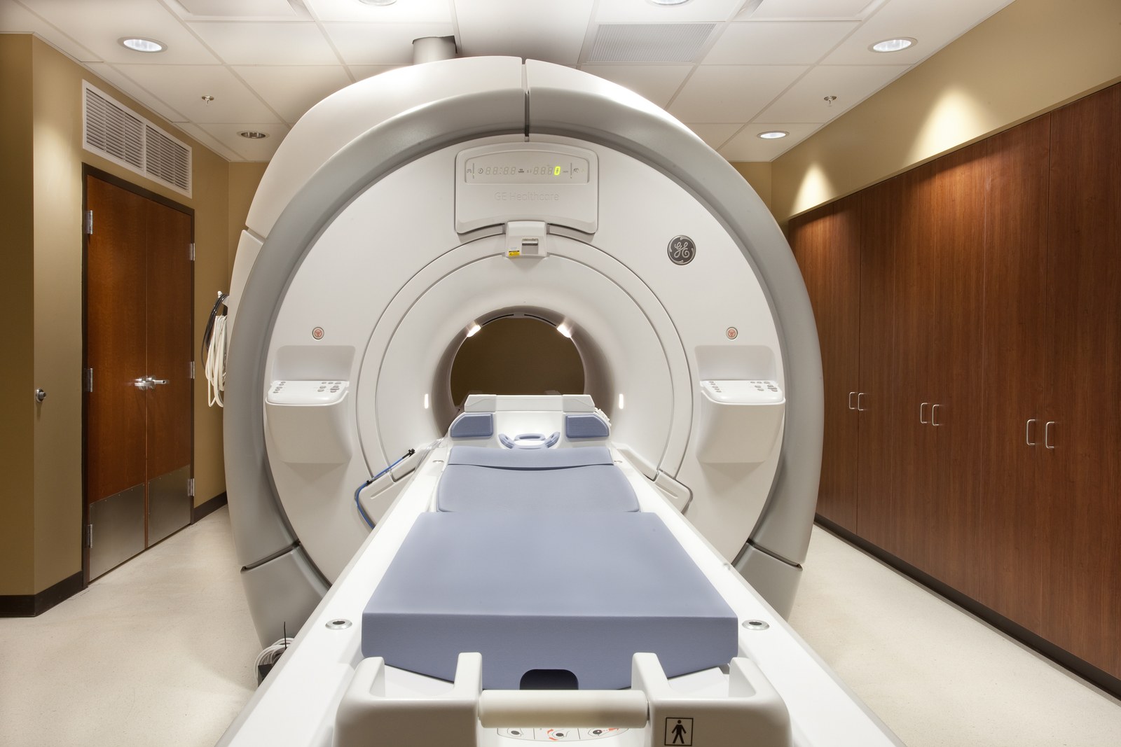
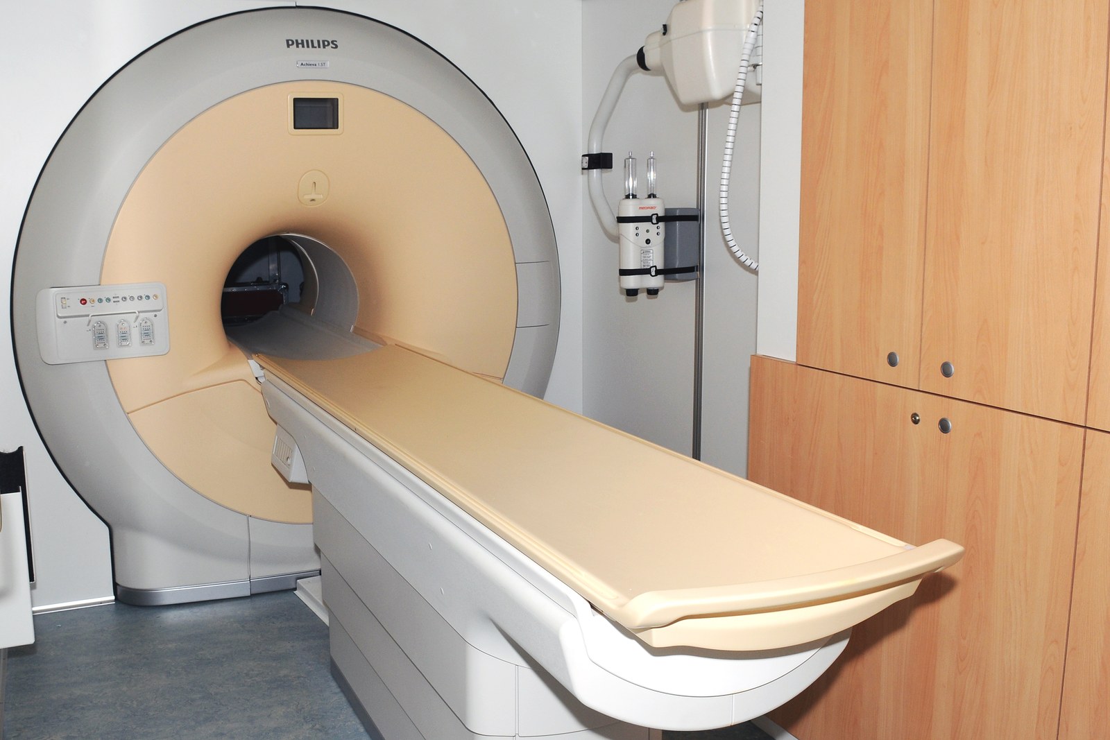
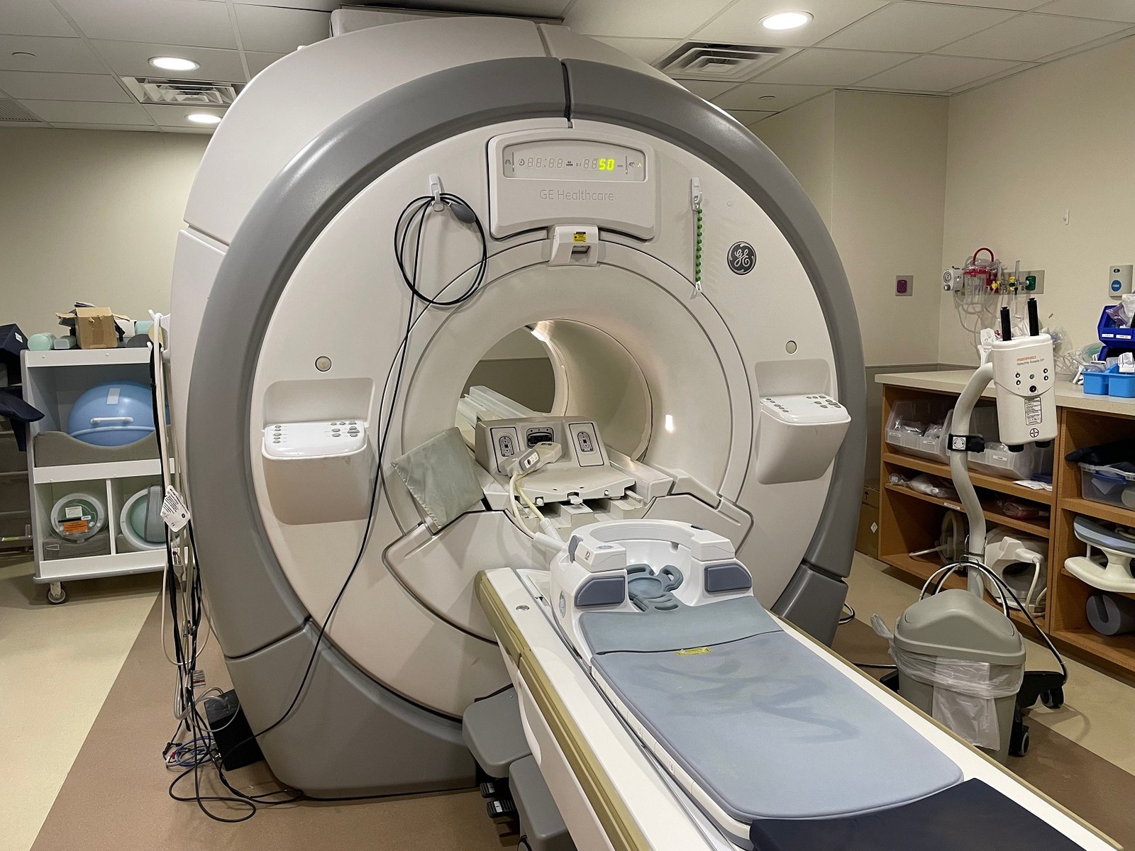
The machines in the photographs on this page include a scanner that appears to be a GE (General Electric) system in a room with wood cabinets, a scanner that appears to be a Philips Achieva-class system (the label on the machine reads Achieva) with peach and cream covers, and another GE Healthcare scanner shown with coils on its table in a clinical room. Model identification from photos is a best guess.

• GE HealthCare (spun off from General Electric in January 2023): SIGNA series (Premier, Architect, Artist, Pioneer, Explorer), Voyager, and SIGNA 7.0 T for research. GE scanners from the 1.5 T Signa era onward were among the first widely installed.
• Siemens Healthineers: MAGNETOM series: Sola and Aera (1.5 T), Vida, Skyra and Prisma (3 T), Terra 7 T, Free.Max and Free.Star (low field, wide bore), and the Cima.X 3 T with very strong gradients.
• Philips: Achieva (older series), Ingenia (1.5 T and 3 T, digital coil-integrated receivers), Ingenia Ambition and the BlueSeal sealed helium magnets, Ingenia Elition 3 T.
• Canon Medical Systems (formerly Toshiba Medical): Vantage Orian (1.5 T) and Vantage Galan (3 T).
• United Imaging (China): uMR 570, 780, 790 and Omega (3 T, 75 cm bore) and a whole-body 5 T system, the uMR Jupiter, reported as cleared in China.
• Hitachi and Fujifilm: Hitachi's medical business, including its open MRI line (permanent magnet and superconducting open systems), was taken over by Fujifilm in 2021 (Fujifilm Healthcare).
• Others: Esaote (dedicated extremity scanners), Hyperfine (portable low field), Fonar (upright and multi-position MRI), Neusoft, Mindray, and Elekta (Unity) and ViewRay (MRIdian) MR-guided radiotherapy machines.

Model lists change often and may be a little dated; check manufacturer pages for current offerings.

SAFETY NOTE

This page is a technical reference, not medical advice. Whether an MRI is needed for a given person, and whether any implant or device makes it unsafe, is a decision for their doctor and the MRI safety staff. Never bring ferromagnetic objects into a scanner room, and never assume a magnet is off.

IN ONE SENTENCE

An MRI scanner uses a strong, always-on superconducting magnet (commonly 1.5 or 3 tesla) to align the hydrogen nuclei in the body, excites them with radio pulses at the Larmor frequency, uses gradient coils to encode where each signal comes from, and Fourier-transforms the received signals into detailed soft-tissue images, with no ionizing radiation, at the cost of long, loud scans and strict magnetic-safety rules.